After reading Making my bookshelves clickable James Coffee Blog, I had a quick idea to experiment with training and deploying CV models. The following is an account of my adventures with CV models for a small bookshelf experiment I wanted to run. Doing experiments, training them and deploying them for a cool nifty little application has been immensely fun and I thought I might just write up a quick piece on the expedition.
Starting “small”
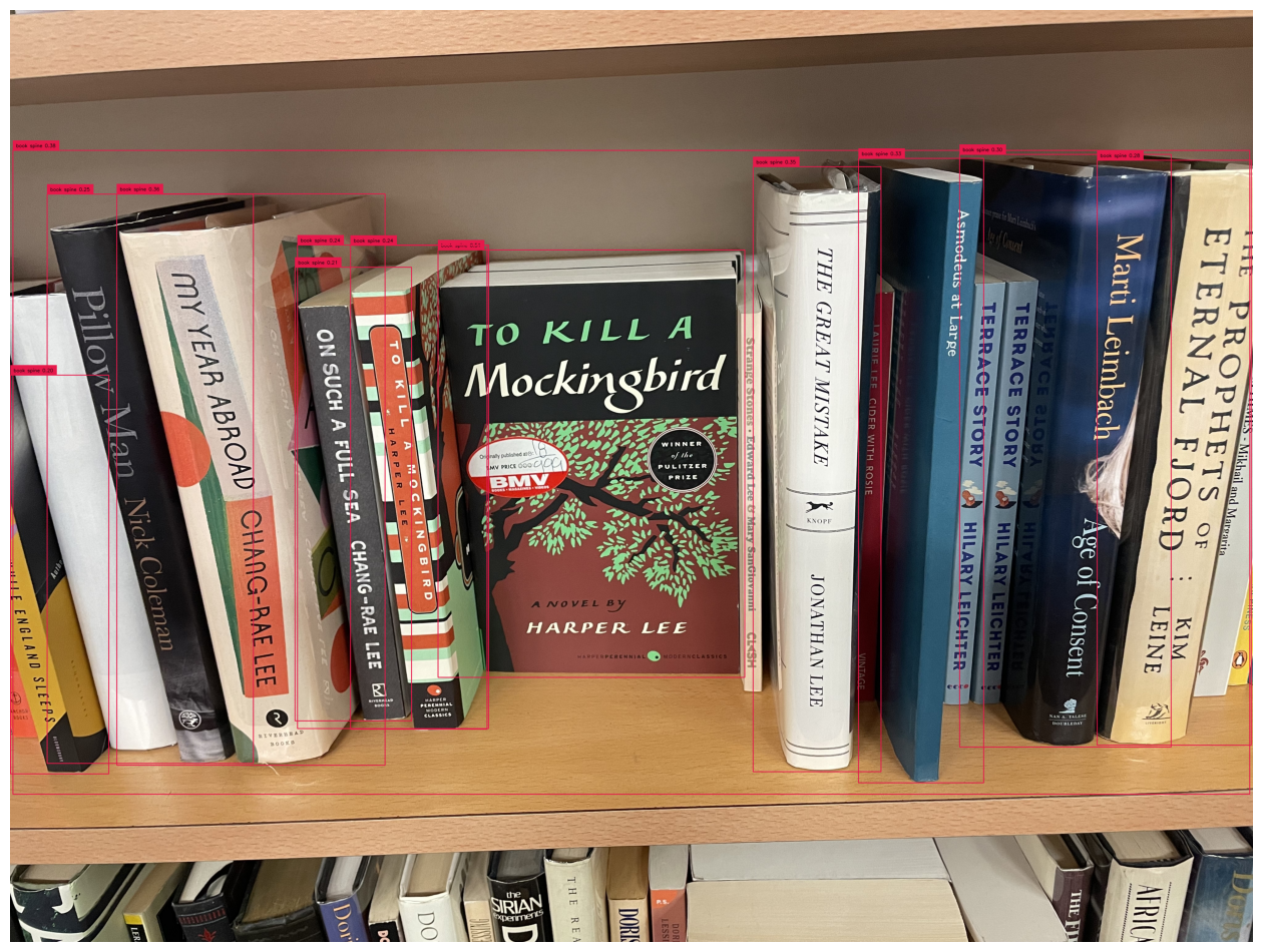
To start off, I tried to replicate James’ experiment using Grounded SAM which is using Grounded DINO for object detection and then SAM on top of the bounding boxes for instance segmentation. This is naturally quite a heavy workflow but very useful to get a grasp on this.
Every journey of a 1000 miles starts with the first step and every great Python adventures starts with a Jupyter notebook. That was exactly ground zero. To replicate James’ blog wasn’t too hard. Had to read some of the documentation on the Grounded DINO + SAM repo by IDEA Research.
Grounding DINO was simple enough. Just had to load the model and then use the predict_with_classes method that they provided.
CLASSES = ['book spine']
BOX_TRESHOLD = 0.2
TEXT_TRESHOLD = 0.15

detections = dino.predict_with_classes(
    image=images[2],
    classes=CLASSES,
    box_threshold=BOX_TRESHOLD,
    text_threshold=TEXT_TRESHOLD
)
print(detections.class_id)
print(detections.confidence)
# annotate image with detections
labels = [
    f"{CLASSES[class_id if class_id is not None else 0]} {confidence:0.2f}"
    for confidence, class_id
    in zip(detections.confidence, detections.class_id)
]

box_annotator = sv.BoxAnnotator()
annotated_frame = box_annotator.annotate(scene=images[2].copy(), detections=detections, labels=labels)

sv.plot_image(annotated_frame, (16, 16))
Then I did the same for SAM.
detections.mask = segment(
    sam_predictor=sam,
    image=cv2.cvtColor(images[2], cv2.COLOR_BGR2RGB),
    xyxy=detections.xyxy
)

# annotate image with detections
box_annotator = sv.BoxAnnotator()
mask_annotator = sv.MaskAnnotator()
labels = [
    f"{CLASSES[class_id]} {confidence:0.2f}"
    for _, _, confidence, class_id, _
    in detections]
annotated_image = mask_annotator.annotate(scene=images[2].copy(), detections=detections)
annotated_image = box_annotator.annotate(scene=annotated_image, detections=detections, labels=labels)

%matplotlib inline
sv.plot_image(annotated_image, (16, 16))
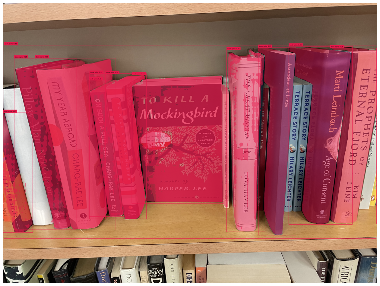
This resulted in about ~ 11s per image with about 75% accuracy. As you'll see below, it doesn't perform the best with slightly narrow or obscured book spines.
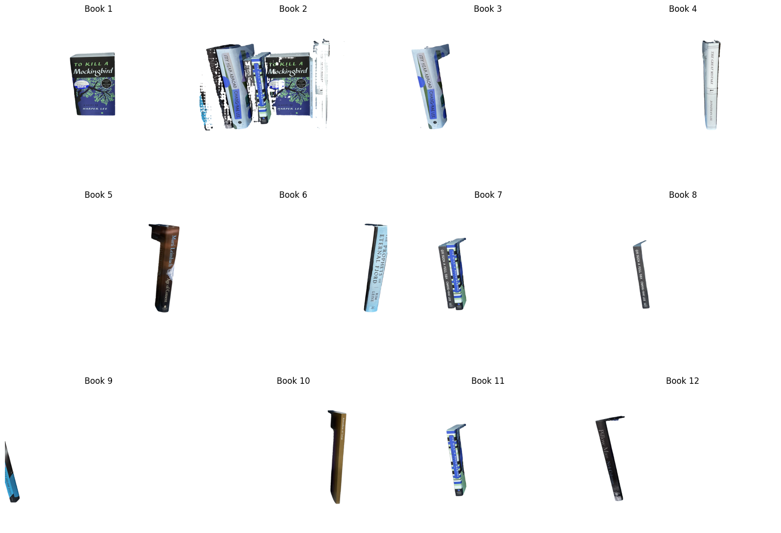
And after getting the instances segmented, I applied a white mask to each of the images and then used GPT-4o Vision for OCR. This I know is kinda like using a nuke to destroy a small house. But I didn't want to go through the process of setting up EasyOCR or anything else. This is what the output looked like.
8%|▊ | 1/12 [00:08<01:31, 8.34s/it]

{"title":"To Kill a Mockingbird","author":"Harper Lee"}

17%|█▋ | 2/12 [00:14<01:08, 6.90s/it]

{"title":"","author":""}

25%|██▌ | 3/12 [00:18<00:53, 5.92s/it]

{"title":"My Year Abroad","author":"Chang-Rae Lee"}

33%|███▎ | 4/12 [00:23<00:42, 5.32s/it]

{"title":"The Great Mistake","author":"Jonathan Lee"}

42%|████▏ | 5/12 [00:27<00:34, 4.96s/it]

{"title":"Age of Consent","author":"Marti Leimbach"}

50%|█████ | 6/12 [00:31<00:27, 4.58s/it]

{"title":"The Prophets of Eternal Fjord","author":"Kim Leine"}

58%|█████▊ | 7/12 [00:35<00:22, 4.49s/it]

{"title":"","author":""}

67%|██████▋ | 8/12 [00:38<00:16, 4.06s/it]

{"title":"On Such a Full Sea","author":"Chang-rae Lee"}

75%|███████▌ | 9/12 [00:42<00:11, 3.84s/it]

{"title":"While England Sleeps","author":"David Leavitt"}

83%|████████▎ | 10/12 [00:45<00:07, 3.69s/it]

{"title":"Asmodeus at Large","author":""}

92%|█████████▏| 11/12 [00:49<00:03, 3.57s/it]

{"title":"To Kill a Mockingbird","author":"Harper Lee"}

100%|██████████| 12/12 [00:52<00:00, 4.34s/it]

{"title":"Pillow Man","author":"Nick Coleman"}
YOLO Shenanigans
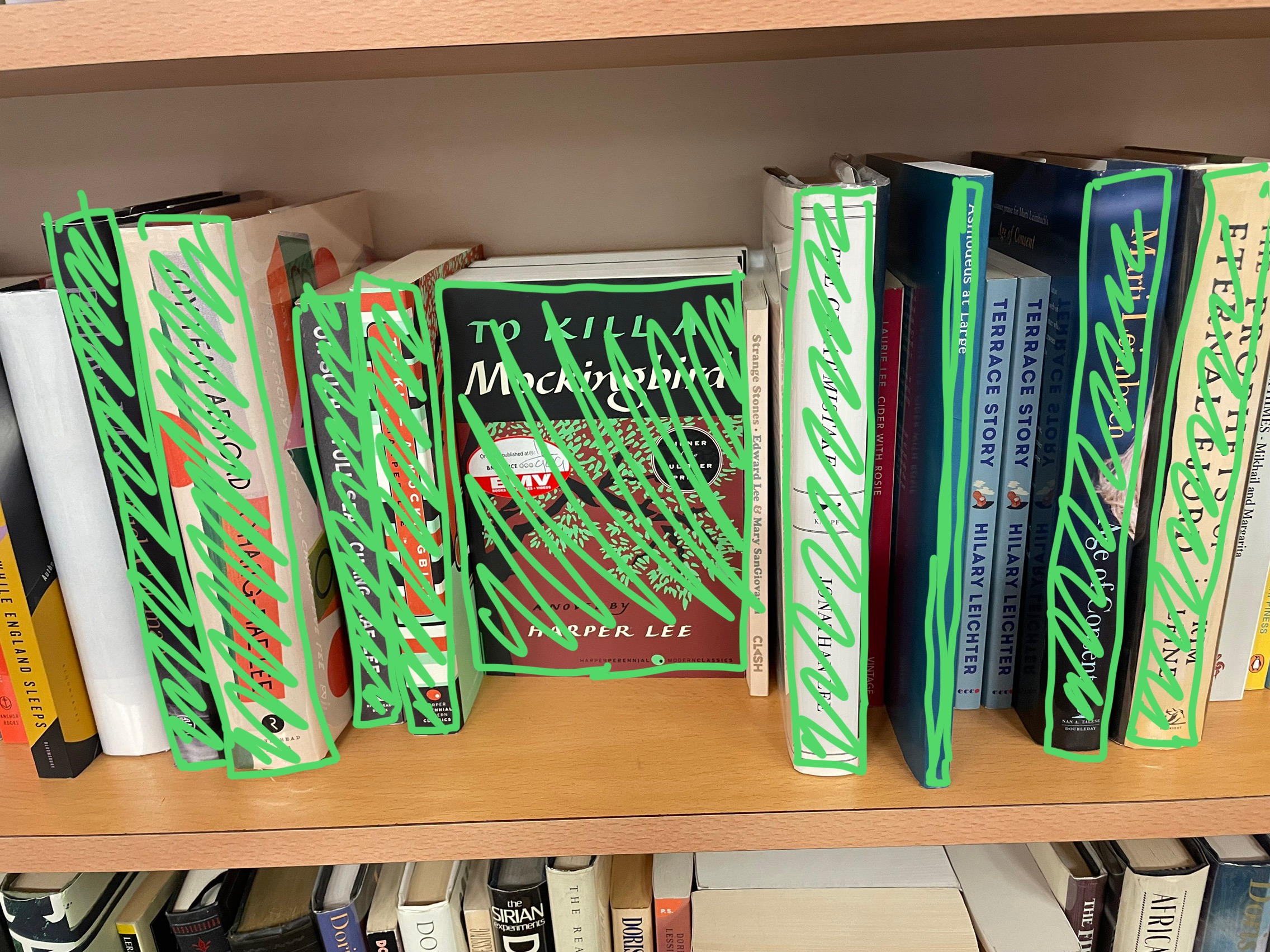
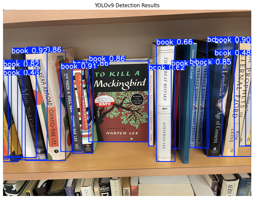
The only problem with the method above was that it was slow since it was a generalized method for object detection. We could get much faster and even better results. For context, in the following image the shaded images were the ones that were correctly identified. Obviously a few were missed. I wanted near perfect recognition. Which shouldn’t be too much to ask for.
So I got to looking elsewhere. Naturally I defaulted to YOLO because that was the fastest model that could deliver the bounding-box object detection that I wanted.
Dataset and model experimentation
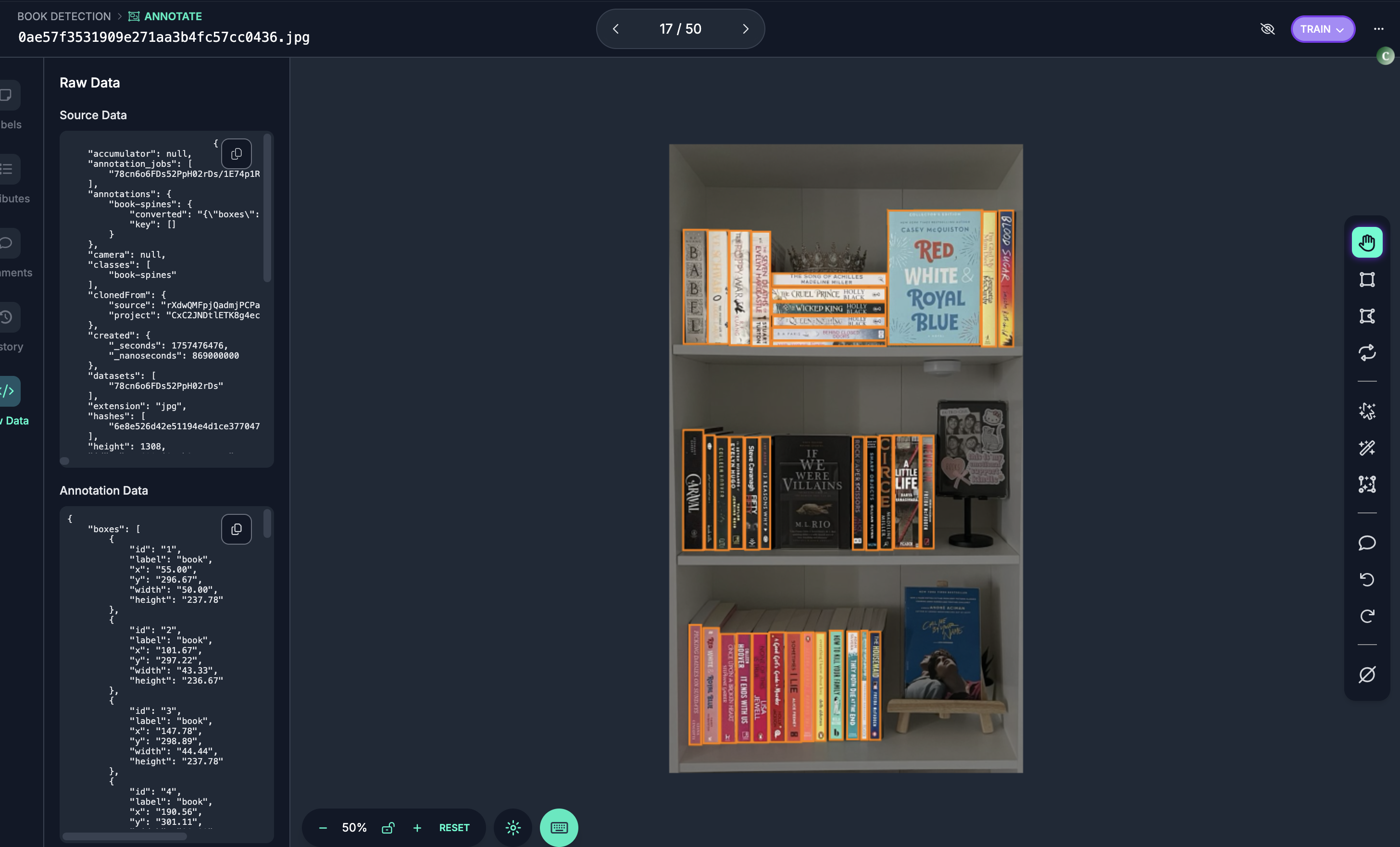
Using Roboflow, I managed to aggregate a dataset for task of object detection of book spines. This required a little bit of scouring on Roboflows website to find such datasets. But once I did, bang! we were in.
I used YOLO9c for this which is slightly long in the tooth but it got the job done.
All that I required was a sleek little Colab with some GPU credits andddd …
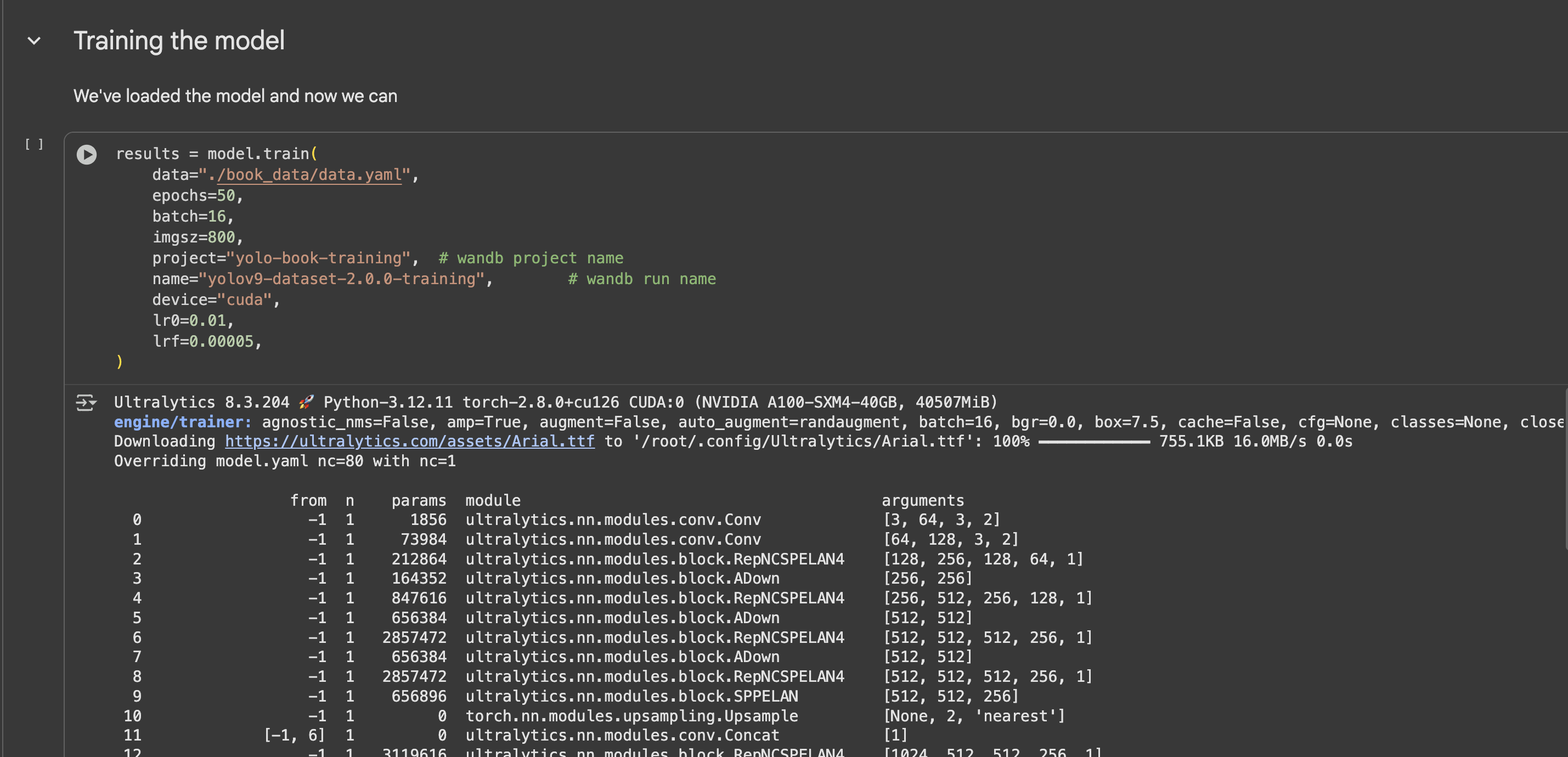
… we got to cooking.
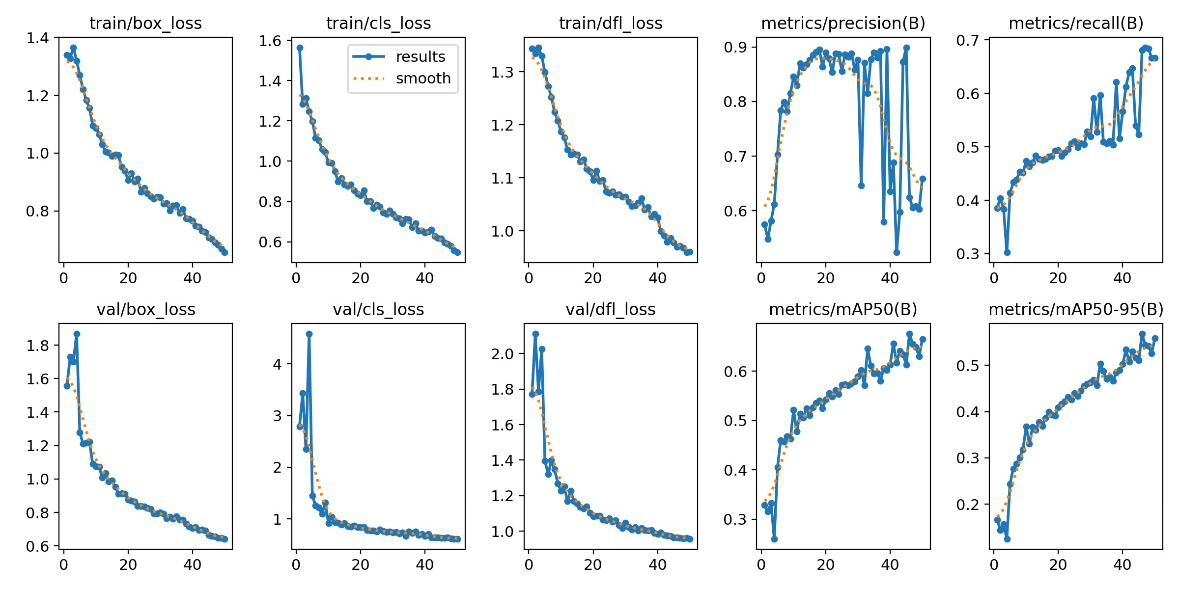
And bada–bing-bada-boom! We nailed it.
I used WandB to track these deployments and display all the metrics. This was my first time using it and was pretty easy and effortless to setup. Gonna be a go to for tracking from now on.
Beware the inference deployments
Now this is something I didn’t consider was going to take so long and in fact shocked me that I took so much time on. Usually when I built a web app in Python, it was a simply Dockerfile with gunicorn as the entrypoint. But this was a different ball game.
- The docker image was too damn high!!. After installing all the dependencies, the docker image size came to 7GB!!!!. SEVEN GIGABYTES!! Why I tried to deploy with Fly.io, it politely told me to rethink my life choices and make a U-turn. After doing a quick Stackoverflow rabbithole, it turns out
opencv-python-headlessis a better option thanopencv-pythonby about 300MB. Furthermoreultralyticsalways installed a version of torch, torchvision which themselves were 2.5 GB cause of the binaries. The patches for all of these was to promptly removeultralytics,torch,torchvisionand use the Dockerfile to install versions with pinned binaries from specific repos.
RUN pip install --no-cache-dir ultralytics --no-deps
- Deploying a trained model requires weights hosting which is its own problem. I needed to have the weights hosted somewhere in an object storage bucket so that I could easily access them. Deploying here automatically after training run #1, #2 and so on was a manual process which did not bring me much joy. But in the name of speed and sanity I swallowed that pill and manually pushed. Not to mentioned fixed the code to autodownload from this “repo”. This had to be better
Takeaways
All in all, working on this project on nights and weekends outside my day job at Martinrea, it took me a week to complete this project. Pretty fun and very exciting. I will be seeing where else this leads me. Some of my important observations for the pipeline
-
Data sanity matters so much more than I thought it did. It should be the first step in preparing your model. My go to when my model is reaching a local minima is that my hyperparameters weren’t configured properly. Something to do with the learning rate scheduling or dropout, etc. But then after stumbling around there for a bit, I decided to take a closer look at the data. (God bless Roboflow) And then started realizing why my model was performing poorly. Lots of the images didn’t match the task distribution I cared about. They were too much at an angle or only looked for book spines instead of just books, etc. Pruning the dataset led to a big spike in the accuracy numbers and when I tested them myself on the little validation dataset I built from real-world photos, they performed much better.
- The data should match the task distribution you finally want it trained for.
- The data should be high quality and not miss out on any obvious labels.
-
Inference deployments are unnecessarily hard for individuals. Maybe I’m missing something here or I didn’t get the memo but to deploy a simple YOLO model that I trained, (using an easy pipeline via FastAPI), I need to
- Build a docker container with all the requirements
- Find somewhere to host the weights so they can be easily downloaded
- Have the code auto download if not present
- Setup a cloud provider with a cheap GPU to run the app
- Deploy the app via the cloud provid All apparently very simple on paper but there’s a lot of hand wringing going on behind the scenes and I haven’t found an atomic way to deploy the models for inference in an instant (atomically via a config file, I mean).
-
Automation and operations matter most in these deployments. A good pipeline is a worth its weight in gold. A bad one is a source of endless grievances. Before developing, it makes the most sense to develop a stable foundation of a pipeline. By this I mean answering the following questions:
- After I train the model, is there an atomic and automated way to deploy the model?
- After I deploy the model, is there an atomic and automated way to monitor the model?
- How can I shrink the time it takes from completed training to traffic?
These are what I've learned so far and there's a ways to go. But this a fun project outside of the default CV stuff from school.
References
[1] Making my bookshelves clickable James Coffee Blog
[2] Model Training with YOLO
[3] Fly.io GPUs
[4] WandB